CAD for Electromagnetic Devices Laboratory Exercise

An introduction to numerical modelling techniques for electromagnetic problems using finite element analysis

Contents

2. Introduction

3. Simulation Results

3.1 Electric Potential

3.2 Magnetic Flux Density

3.3 Magnetic Flux Density For Single Conductor

3.4 Finite Difference vs Finite Element

3.5 Comb Drive Micro Actuator

3.6 Magnetic Circuit

4. Discussion

Finite element analysis (FEA) is the ‘modelling of products and systems in a virtual environment, for the purpose of solving potential (or existing) structural or performance issues.’ (1) FEA is the practical application of the finite element method (FEM), a numerical technique for ‘approximating solutions to boundary value problems for partial differential equations’ (2) which cannot be solved analytically. This method works by separating a large system into smaller parts called finite elements, known as discretization (3). The simple equations governing these finite elements are accumulated to form an overall system of equations for the problem, which FEM uses to approximate a solution.

Computational Electromagnetics is ‘the process of modelling the interaction of electromagnetic fields with physical objects and the environment.’ (4) The electromagnetic analysis that this involves is based on solving Maxwell’s equations subject to given boundary conditions. Maxwell’s equations can be expressed in general differential form and therefore the solutions to electromagnetic problems governed by these equations can be modelled and solved using FEM. (5)

The electromagnetic problems outlined in this report have been modelled and approximated in two-dimensional space using the finite element program ‘pdetool’ in MatLab. This is done through the use of linear triangular elements.

3.1 Electric Potential

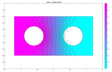The aim of this experiment was to model the electric potential between two circular metallic conductors of radius 30 cm and centre distance 120cm. The left and right conductors were subject to Dirichlet boundary conditions and given potentials of 1 and -1 respectively. The enclosed area was modelled using the Neumann boundary condition (6) and the current source set to 0. The following model was observed:

The purple to blue shading demonstrates the varying electric potential across the model, with V = 0 at the midpoint of the two conductors as anticipated due to the equation… The electric field is visualised through the red arrows, confirming the expectation that the current would flow from the positively charged conductor to the negatively charged conductor.

3.2 Magnetic Flux Density

This experiment aimed to model the magnetic field between two cylindrical, current-carrying conductors of radius 5cm and centre distance of 60cm. The magnetic permeability of both conductors was set to and the current density set to 1 and -1 respectively. The enclosed area was modelled using Dirichlet boundary conditions with magnetic potential set to 0, and the magnetic potential and current density set to and 0 correspondingly. The following model was observed:

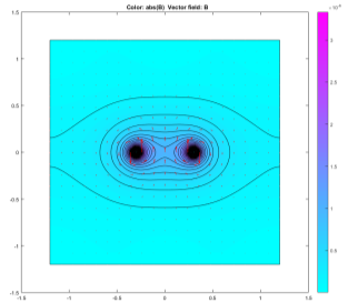
The red arrows show the direction of the magnetic field at certain points, while the shading demonstrates the magnitude of the magnetic flux density, clearly highlighting that the strength of magnetic flux decreases with distance away from the conductors.

The current in each conductor is given by the equation , where J is the current density and A is the cross sectional area of the conductor. Using this equation yields a current of 7.85mA for the left conductor and -7.85mA for the right conductor.

3.3 Magnetic Flux Density For Single Conductor

The experiment from 3.2 was then replicated using a single, circular, current-carrying conductor of radius 0.2cm. The boundary conditions for the enclosed area remained the same while, for the conductor, magnetic permeability was set to and current density to 1. The following model was observed:

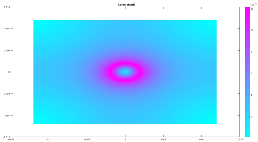
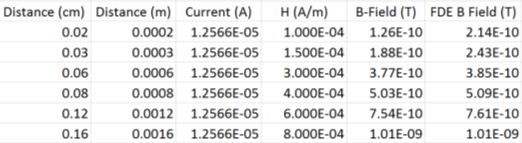
The magnetic flux density was then measured from the FEM model for a number of distances and compared with results calculated from theory; this comparison can be found in table 1 below.

3.4 Finite Difference vs Finite Element

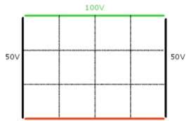For this electrostatic model, a 16cm x 12cm square was plotted to represent four electric diodes of differing electric potential, shown in figure 4.

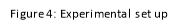
The dielectric permittivity of the electric diodes was set to 1 and the electric potential and electric field for the system was modelled as shown below:

The variation of electric field between the positive and negative diodes is represented through the shading and the electric field lines are shown in black.

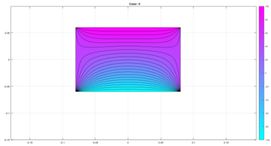
Values for the electric potential at particular geometric coordinates were then measured from the FEM model and compared against the results calculated from FDM; this comparison can be found in table 2.

3.5 Comb Drive Micro Actuator

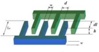This experiment aimed to model the electric field distribution of a voltage controlled, comb-drive, electrostatic micro-actuator, consisting of a movable comb and a fixed comb, with the latter containing four fingers. The dimensions of the comb were specified as follows: w=1, d=1, dl=0.6 and Lc=3 (all figures are in mm) and explained through figure 6:

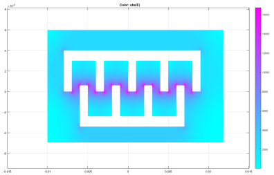
The movable comb was given a potential of 5V and the fixed comb a potential of -5V to simulate a 10V applied voltage. The electric potential of the enclosed area was set to 0 and the space charge density to 0 as well. The following model, demonstrating electric field distribution, was observed:

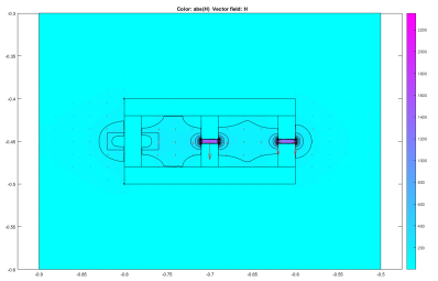
3.6 Magnetic Circuit

A model for an electromagnet was created as shown in figure 8 below:

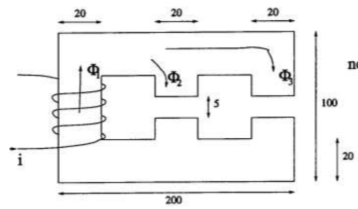
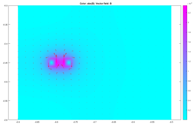
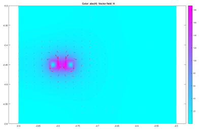
The magnetic permeability of the iron was set to 500 and current density 0. The coil was represented in the model by two rectangles either side of where the coil appears in figure 6, one with positive and one with negative current density. Given that the current in the coil is 10 A-turns, the current density is given by the equation, where A is equal to the area of the approximated coil. The magnetic permeability of both the ‘coil’ and the enclosed area were set to and models for the magnetic flux density and magnetic field were achieved. These are shown below:

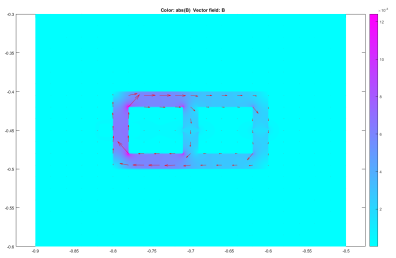
The experiment was then altered to model the effects of the coil if the material of the magnet was plastic, with a relative permeability of 1, and therefore the magnetic permeability of the magnet was set to . All the other values remained constant. The magnetic flux density and magnetic field were then found and are shown below: