Information Theory and Thermodynamics
| ✅ Paper Type: Free Essay | ✅ Subject: Physics |
| ✅ Wordcount: 1474 words | ✅ Published: 11 Sep 2017 |
In order to develop better tools, machines and technology we have had to develop our understanding of the physical world. This has allowed us to construct machines that are more capable than those preceding it.
The French scientist Carnot was studying machines and was trying to understand how to make them better and more efficient. As part of his studies he calculated the maximum efficiency of any machine and was able to relate this to temperature. Carnot’s idea was to simplify the machine to its simplest form (this generality that makes it universal) and analyse that – Carnot knew that machines of the time (and of today) work as a result of a temperature difference across the machine. In his time it was obvious, fire produced steam which turned a turbine that did work; today is not too different, all of our machines still need a temperature difference to make them work, however the temperature difference driving the machines may be at some distance, for example a power station producing electricity. Even wind, and solar require temperature differences to work.
Analysing these machines further lead to concepts that we, perhaps, take for granted: work, power and energy notable examples. Whilst working on these concepts Boltzmann came up ideas that grew into statistical thermodynamics. It was extended and correctly describes a whole range of phenomena.

The idea of thermodynamics is to relate various physical properties of a substance to the “bulk” behaviour of the constituent parts within.
Microstates and Macrostates:
Boltzmann realised that by knowing the number of different states that a system could be in and the number of configurations that each state would enable him to work out the probability of a particular state occurring. And that on average when something is observed it is more likely to be found in one of its more probable states. Many systems have lots of moving components and this means that over time a system will have “evolved” into a more probable state. This may now seem obvious, but it hadn’t been pointed out explicitly at the time.
A Macrostate is the global state of a system. For example if we consider a box with red, blue and green balls a possible macrostate might be to find all of the red balls are in the bottom left corner, whilst all of the others are randomly distributed in the rest of the box. Another example of a macrostate might be that the total electrical charge of block could be  Coulombs.
A Microstate is one particular configuration of the system that produces a macrostate. In the balls example if the balls are identical apart from colour we can permute the balls with the same colour amongst themselves and end up with different microstates. An example with the charged block might be that we have 4 particles each with charge  as one microstate, and another might be to have 1 particle with and another with
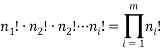
Below is a figure that represents a hypothetical macrostate of three colours of balls three particular microstates that can be used to achieve it. In the leftmost diagram we have a macrostate with all of the red balls in the bottom left corner, the other diagrams show different permutations of the balls that also achieve the desired macrostate.

In order to calculate the probability of this state we would need to know how many combinations of it there are. This is a simple counting argument: we have 1 way of putting the green ball in its spot, two ways of putting the blue balls in their position and 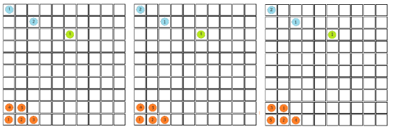
 ways of arranging (we can pick any of the 5 to go in the corner, then any of the remaining 4 to go next to that, then any of the remaining 3 etc). There are a total of 8 balls and so the
In general if there are  objects we have
  possible arrangements; if we also have
  different “types” and if
  of them are of type 1 (say red),
  are of type 2 and
  are of type
  then we can find the total number of permuted arrangements with:
We can use these two facts to calculate the number of “accessible” microstates of type , this is called the “weight” of the  microstate and is denoted by,
  :
:

The weight of a microstate is proportional to the probability of the system being in it. So one way to calculate the probability of being in the state is via:

where the summation is over the weights of all the other possible microstates.
A handy way to view a microstate is with a pack of cards (Birks bath), in a pack of playing cards the statistical weight of a club is 13 since there are 13 of then the statistical weight of a queen is 4. The probability of selecting a club card is  the chances of picking out a club are
  times greater than picking out a queen. The statistical weight of the queen of hearts is 1.
There is one obvious constraint that can always be imposed and that is that the total number of particles is the sum of the number of particles in each state:

We can impose other constraints on the system as they are required later. Because the particles of each type are identical it is natural to assign a probability that a randomly selected particle is of type, , as:

We are also able to define an “Expectation” value for the system. If we were interested in the average occupancy of each of the types we would have:

which would represent the average occupancy of each type. If we were interested in the charge (or energy (I shall use  for either) we would similarly have:

Let us take some examples and compute the statistical weights, average occupancy and average energy (represented by the value of the type index e.g. if  , the energy would be two units). I shall consider that the “atoms” are all identical apart from the energy that they have and that a macrostate is the same for each. For the first case let us assume that we have 5 atoms and the macrostate corresponds to an energy of 5 units. The table below shows that (for example) the microstate 3 has a weight of 20, this means that there are 20 microstates with the occupancy levels given that correspond to the macrostate
  We can tabulate the various combinations as below:
|
microstate number |
Occupancy of type i |
“weight” |
probability |
|||||
|
n0 |
n1 |
n2 |
n3 |
n4 |
n5 |
|||
|
1 |
4 |
0 |
0 |
0 |
0 |
1 |
5 |
0.0397 |
|
2 |
3 |
1 |
0 |
0 |
1 |
0 |
20 |
0.1587 |
|
3 |
3 |
0 |
1 |
1 |
0 |
0 |
20 |
0.1587 |
|
4 |
2 |
2 |
0 |
1 |
0 |
0 |
30 |
0.2381 |
|
5 |
2 |
1 |
2 |
0 |
0 |
0 |
30 |
0.2381 |
|
6 |
1 |
3 |
1 |
0 |
0 |
0 |
20 |
0.1587 |
|
7 |
0 |
5 |
0 |
0 |
0 |
0 |
1 |
0.0079 |
|
totals |
15 |
12 |
4 |
2 |
1 |
1 |
126 |
1 |
|
Average occupancy |
2.222 |
1.389 |
0.794 |
0.397 |
0.159 |
0.040 |
||
Table 3.1: Table showing occupancy levels for a 5 atom system with a macrostate of 5.
This table was generated by finding all of the numbers that sum (in this case) to 5 which is the macrostate. It shows the number of atoms with a particular energy in the columns headed , the statistical weight of each microstate is in the “weight” column, the probability column next to it shows the probability of randomly selecting this microstate from a given macrostate (in this case 5 atoms and a total energy of 5). The row titled average occupancy shows the expected occupancy of an energy level of type , calculated from the table. Looking at the table there are two equally most likely microstate arrangements. The first of these corresponds to  and
and  , both occurring with a probability of 0.238.
Another possible macrostate is listed below, this time we have 7 atoms and an energy of 7 units. The headings of the table are the same as in the previous example. We can see that the weight of the most probable microstate is 420 and that we have a probability of 0.245 of randomly selecting one of them. The occupancy levels are:
|
microstate |
occupancy of type i |
weight |
probability |
|||||||
|
n0 |
n1 |
n2 |
n3 |
n4 |
n5 |
n6 |
n7 |
|||
|
1 |
6 |
0 |
0 |
0 |
0 |
0 |
0 |
1 |
7 |
0.004 |
|
2 |
5 |
1 |
0 |
0 |
0 |
0 |
1 |
0 |
42 |
0.024 |
|
3 |
5 |
0 |
1 |
0 |
0 |
1 |
0 |
0 |
42 |
0.024 |
|
4 |
5 |
0 |
0 |
1 |
1 |
0 |
0 |
0 |
42 |
0.024 |
|
5 |
4 |
2 |
0 |
0 |
0 |
1 |
0 |
0 |
105 |
0.061 |
|
6 |
4 |
1 |
1 |
0 |
1 |
0 |
0 |
0 |
210 |
0.122 |
|
7 |
4 |
1 |
0 |
2 |
0 |
0 |
0 |
0 |
105 |
0.061 |
|
8 |
4 |
0 |
2 |
1 |
0 |
0 |
0 |
0 |
105 |
0.061 |
|
9 |
3 |
3 |
0 |
0 |
1 |
0 |
0 |
0 |
140 |
0.082 |
|
10 |
3 |
2 |
1 |
1 |
0 |
0 |
0 |
0 |
420 |
0.245 |
|
11 |
3 |
1 |
3 |
0 |
0 |
0 |
0 |
0 |
140 |
0.082 |
|
12 |
2 |
4 |
0 |
1 |
0 |
0 |
0 |
0 |
105 |
0.061 |
|
13 |
2 |
3 |
2 |
0 |
0 |
0 |
0 |
0 |
210 |
0.122 |
|
14 |
1 |
5 |
1 |
0 |
0 |
0 |
0 |
0 |
42 |
0.024 |
|
15 |
0 |
7 |
0 |
0 |
0 |
0 |
0 |
0 |
1 |
0.001 |
|
totals |
51 |
30 |
11 |
6 |
3 |
2 |
1 |
1 |
1716 |
1 |
|
Average occupancy |
3.231 |
1.885 |
1.028 |
0.514 |
0.228 |
0.086 |
0.024 |
0.004 |
||
Table A3 2: a seven atom system with a total energy of seven

A final example consists of a system of 10 atoms and a total energy of 9. As will be readily seen as the number of atoms and the energy increases the number of microstates corresponding to a given macrostate increases so does the size of the table. It was quite difficult to work out the number of combinations of energy that could occur and I wouldn’t want to do it again for larger tables. In the next part we shall use the method of Lagrange multipliers to massively simplify the calculations for the probabilities and expectations. For the case of 10 atoms and an energy of 9 units.
We see that the most probable microstates have the following occupancy levels:

The most probable microstate has a probability of 0.1555, but there is another microstate that is only slightly less probable (a probability of 0.1300) and this has occupancy levels of:

The two least likely microstates are the following:


Both have a probability of 0.0002 which is very small indeed. Table 3 is below:
|
d |
occupancy of each type i |
“weight” |
probability |
|||||||||
|
n0 |
n1 |
n2 |
n3 |
n4 |
n5 |
n6 |
n7 |
n8 |
n9 |
|||
|
1 |
9 |
0 |
0 |
0 |
0 |
0 |
0 |
0 |
0 |
1 |
10 |
0.000205677 |
|
2 |
8 |
1 |
0 |
0 |
0 |
0 |
0 |
0 |
1 |
0 |
90 |
0.00185109 |
|
3 |
8 |
0 |
1 |
0 |
0 |
0 |
0 |
1 |
0 |
0 |
90 |
0.00185109 |
|
4 |
8 |
0 |
0 |
1 |
0 |
0 |
1 |
0 |
0 |
0 |
90 |
0.00185109 |
|
5 |
8 |
0 |
0 |
0 |
1 |
1 |
0 |
0 |
0 |
0 |
90 |
0.00185109 |
|
6 |
7 |
2 |
0 |
0 |
0 |
0 |
0 |
1 |
0 |
0 |
360 |
0.00740436 |
|
7 |
7 |
1 |
1 |
0 |
0 |
0 |
1 |
0 |
0 |
0 |
720 |
0.014808721 |
|
8 |
7 |
1 |
0 |
1 |
0 |
1 |
0 |
0 |
0 |
0 |
720 |
0.014808721 |
|
9 |
7 |
1 |
0 |
0 |
2 |
0 |
0 |
0 |
0 |
0 |
360 |
0.00740436 |
|
10 |
7 |
0 |
2 |
0 |
0 |
1 |
0 |
0 |
0 |
0 |
360 |
0.00740436 |
|
11 |
7 |
0 |
1 |
1 |
1 |
0 |
0 |
0 |
0 |
0 |
720 |
0.014808721 |
|
12 |
7 |
0 |
0 |
3 |
0 |
0 |
0 |
0 |
0 |
0 |
120 |
0.00246812 |
|
13 |
6 |
3 |
0 |
0 |
0 |
0 |
1 |
0 |
0 |
0 |
840 |
0.017276841 |
|
14 |
6 |
2 |
1 |
0 |
0 |
1 |
0 |
0 |
0 |
0 |
2520 |
0.051830522 |
|
15 |
6 |
2 |
0 |
1 |
1 |
0 |
0 |
0 |
0 |
0 |
2520 |
0.051830522 |
|
16 |
6 |
1 |
2 |
0 |
1 |
0 |
0 |
0 |
0 |
0 |
2520 |
0.051830522 |
|
17 |
6 |
1 |
1 |
2 |
0 |
0 |
0 |
0 |
0 |
0 |
2520 |
0.051830522 |
|
18 |
6 |
0 |
3 |
1 |
0 |
0 |
0 |
0 |
0 |
0 |
840 |
0.017276841 |
|
19 |
5 |
4 |
0 |
0 |
0 |
1 |
0 |
0 |
0 |
0 |
1260 |
0.025915261 |
|
20 |
5 |
3 |
1 |
0 |
1 |
0 |
0 |
0 |
0 |
0 |
5040 |
0.103661045 |
|
21 |
5 |
3 |
0 |
2 |
0 |
0 |
0 |
0 |
0 |
0 |
2520 |
0.051830522 |
|
22 |
5 |
2 |
2 |
1 |
0 |
0 |
0 |
0 |
0 |
0 |
7560 |
0.155491567 |
|
23 |
5 |
1 |
4 |
0 |
0 |
0 |
0 |
0 |
0 |
0 |
1260 |
0.025915261 |
|
24 |
4 |
5 |
0 |
0 |
1 |
0 |
0 |
0 |
0 |
0 |
1260 |
0.025915261 |
|
25 |
4 |
4 |
1 |
1 |
0 |
0 |
0 |
0 |
0 |
0 |
6300 |
0.129576306 |
|
26 |
4 |
3 |
3 |
0 |
0 |
0 |
0 |
0 |
0 |
0 |
4200 |
0.086384204 |
|
27 |
3 |
6 |
0 |
1 |
0 |
0 |
0 |
0 |
0 |
0 |
840 |
0.017276841 |
|
28 |
3 |
5 |
2 |
0 |
0 |
0 |
0 |
0 |
0 |
0 |
2520 |
0.051830522 |
|
29 |
2 |
7 |
1 |
0 |
0 |
0 |
0 |
0 |
0 |
0 |
360 |
0.00740436 |
|
30 |
||||||||||||
Cite This Work
To export a reference to this article please select a referencing stye below:
Related Services
View all


DMCA / Removal Request
If you are the original writer of this essay and no longer wish to have your work published on UKEssays.com then please click the following link to email our support team:
Request essay removal